


Welcome to Lab 3 of the Finetuning Sessions!
In today's lab, we’re going to run more finetuning experiment — specifically, LoRA finetuning.
📕 If you haven't read Lesson 3's article, make sure to review it before going forward!

The shift from Full Finetuning (FFT) to Parameter-Efficient Finetuning (PEFT) has redefined how we approach model adaptation. At the center of this paradigm shift is Low-Rank Adaptation (LoRA). While often pitched simply as a "cheaper way to fine-tune", treating LoRA as a black box leaves performance on the table.
So, today, we are going deep.
We will dissect the exact mechanics of how LoRA slashes the "fixed costs" of memory during training, how to navigate its highly sensitive hyperparameter space, and how the concept of Multi-LoRA is revolutionizing both training and deployment.
The "Fixed Costs" of GPU Memory

Residual states consist of activations and temporary buffers, which scale dynamically with your sequence length and batch size.
But the true bottleneck for massive models lies in the model states—the "fixed costs" of training. Model states include the parameter weights themselves, the gradients, and the higher-order optimization quantities (like momentum and variance in the Adam optimizer).
If we perform Full Finetuning (FFT) on a 7-billion parameter model using the Adam optimizer in single precision (FP32), the math is punishing. You need 16 bytes per parameter:
4 bytes for the master weight.
4 bytes for the gradient.
8 bytes for the optimizer states (4 for momentum, 4 for variance).
For a 7B model, these fixed model states alone consume 112 GB of VRAM. This completely prices out consumer hardware!
LoRA fundamentally alters this equation by freezing the original weights and only calculating gradients and optimizer states for a tiny fraction of injected low-rank matrices.
If we assume LoRA adds just 1% of trainable parameters (e.g., ~70M parameters) and we store the frozen base model in bfloat16 (2 bytes per parameter), the fixed costs plummet:
Base weights (frozen):
2 bytes * 7B = 14 GBLoRA trainable parameters (Adam, FP32):
16 bytes * 0.07B = 1.12 GB
The total memory required for model states drops from 112 GB to roughly 15.12 GB.
By neutralizing the gradient and optimizer footprint for 99% of the network, LoRA turns finetuning from a datacenter-scale problem into a workstation-scale task.
Navigating the Hyperparameter Maze
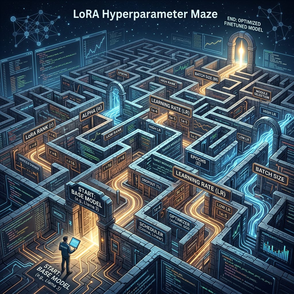
The architectural simplicity of LoRA—where the weight update is parameterized as ΔW=BA—hides a complex optimization landscape.
Achieving parity with full finetuning requires strict adherence to hyperparameter best practices.
➤ Target Modules
Early LoRA implementations exclusively targeted the query (W_q) and value (W_v) projection matrices in the self-attention mechanism.
However, exhaustive empirical studies have shown that "attention-only" LoRA heavily underperforms. The best practice is now to apply LoRA to all major linear layers, specifically including the Multi-Layer Perceptron (MLP) layers (gate, up, and down projections).
The MLP layers house the vast majority of a model’s parameters, and targeting them is absolutely essential for driving domain specialization and complex reasoning.
➤ Rank (r) and the Alpha (α) Scaling Factor
The rank (r) determines the dimensionality of your bottleneck.
While tiny ranks (4 or 8) are sufficient for simple natural language tasks, complex domains like coding or mathematics require higher capacity, often necessitating ranks of 64, 128, or 256.
However, simply increasing the rank without adjusting the scaling factor (α) will cause the model to collapse into suboptimal, low-rank solutions.
The LoRA update is scaled by the term α / r. A mathematically sound and highly recommended heuristic is to maintain α = 2r (or at least α = r ). Keeping α fixed (e.g., α=8) while scaling up rank drastically reduces the effective rank of the updates, causing the model to underutilize its capacity and suffer from catastrophic forgetting.
➤ Learning Rate: The 10x Rule
Perhaps the most counterintuitive aspect of LoRA is its learning rate dynamics.
LoRA requires a learning rate that is generally an order of magnitude (10x) higher than what you would use for full finetuning.
For example, if the optimal learning rate for FFT is 2e-5, the optimal LoRA learning rate will likely sit around 2e-4. Because LoRA initializes matrix B to zero, updates at the beginning of training have an incredibly small impact on the network's outputs, necessitating this much more aggressive learning rate schedule to achieve convergence.
